
Predicting subscriber lifetime value using survival analysis
In 2011, I got a Spotify premium subscription as a present to myself for getting a new job. That must be roughly £1200 to date, which for 11 years of ad-free music seems like a bargain.
At the time, signing up to direct debits beyond rent and bills seemed like a lavish extravagance. But now a whole clatter of them leave my account every month. I’ve got the usual Netflix, Prime (Apple TV, Disney, NowTV, other strangely named Amazon ones I don’t remember signing up for), as well as I assume the more unusual fermented goat milk and dog gps tracker.
For obvious reasons it’s an appealing business model. Once acquired, customers generate a regular stream of revenue for as long as they’re retained. The ordeal of cancelling adds some ‘stickiness’, and user data gathered can be used to target offers and recommendations.
But as competition intensifies and the cost of living crisis squeezes household budgets, it’s more important than ever to understand the numbers.
Customer lifetime value (CLV) is the amount of revenue a newly acquired customer will generate over the course of their time as a customer, net of costs. It is a crucial metric for subscription-based businesses to understand. CLV informs how much should be spent on customer acquisition and retention, it determines how you set price levels and how to structure product bundles.
In this post I will describe how to model subscriber lifetime value using techniques borrowed from medical statistics. There are numerous alternative approaches, but this one is intuitive, data-light, fast to implement and accurate.
The components of CLV
We can break down the CLV calculation into a few components, each of which can be estimated using data.
This is the classic formulation. It is a summation over time - in this case from acquisition time = 0 to an arbitrarily chosen point in the future T. The part on the top of the fraction is the money. V is the value or price paid by the subscriber every time period t. K is the cost of servicing and retaining the subscriber each month. Both of these values can be estimated using models.
Here though I'm focusing on S, the survival probability. This tells you the probability the subscriber is still a subscriber at different times in the future.

d is the discount rate. This part of the formula converts future values into present values, reflecting the fact that money earned today is worth more than the same amount earned in the future.
The survival function
Survival analysis is a branch of statistics concerned with modelling the time until some event of interest occurs. This could be anything from death, to product failure, to an insurance claim. In this case, it is a subscription cancellation.
The primary objective of survival analysis is to estimate the survival function.

The y-axis gives the probability that the event of interest has not yet happened by the time point on the x-axis. It is the complement of the cumulative probability distribution function. We can plug these probabilities into the CLV formula, along with values for the price, cost and discount rate.
Censored data
At its core, survival analysis is about how to estimate a survival function with censored data. Censored data is where, for a subset of observations, the final event time is unknown because it hasn’t occurred yet.

In this visualisation each row represents an individual. The dot on the left represents the time they took out their subscription and the dot on the right represents the latest timestamp we have for that individual. For the red dots that timestamp is their cancellation time. These observations are not censored. The three green dots are still active subscribers and their timestamp is their latest renewal date. Simply ignoring these censored data points (or ignoring the fact they’re censored) will bias our survival function estimates.
But this is the only information we need to fit a survival curve: the duration each individual has been a subscriber for and whether they’re still active or not.
Fitting a curve
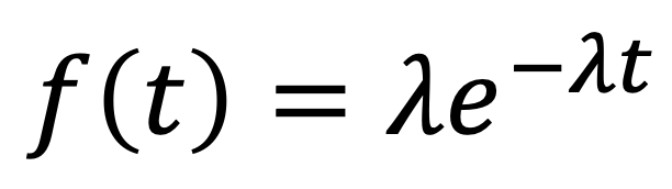
To fit a (parametric) survival model, we first choose a functional form, for example the exponential distribution. This distribution gives the probability the event of interest will occur at different times.
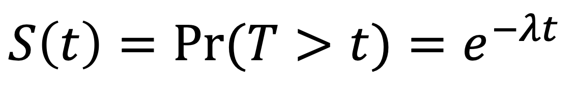
From this we can derive a survival function (by integrating over the pdf above from time t to infinity):
In this particular case we have only one parameter to estimate, which we can do using maximum likelihood estimation (MLE).
To estimate a parameter using MLE, we first construct a likelihood function, which gives the joint probability of observing some data given some parameter value. And then by one means or another find the parameter value that maximises that probability.
Cancelled subscribers are not censored - we know the end date of their subscription. These contribute the probability density f(t) to the likelihood function. For active subscriptions, all we know is that they have not cancelled yet. These observations contribute the survival probability S(t) to the likelihood function. It is in this way that survival analysis handles censored data.
‘…customers don’t behave like uranium…’ - Berry & Linoff (2004)
But there is a problem with our exponential model: it doesn’t fit the data at all well. The reason is that it implies a constant retention rate - i.e. that the probability an active subscriber at time t renews into time t+1 is constant for all t.
While this may or may not be true at an individual level, at a cohort level it certainly isn’t. High churn / low retention subscribers drop out early, leaving only lower churn / high retention subscribers. This ‘sorting effect’ means the average cohort-level retention rate should increase with tenure. And it turns out this trips up any simple parametric model, not just the exponential - in the words of Berry & Linoff (2004) ‘...parametric approaches do not work…’.
The geometric-beta model
To analyse this properly, we need to model subscriber differences explicitly. Fader and Hardie (2006) provide a neat approach for this called the (shifted) geometric-beta model.
In this model we assume 1) that at each renewal opportunity a subscriber will cancel with probability theta, and 2) that there is heterogeneity in theta across subscribers.
1) is captured by a geometric distribution. This gives the probability of ‘failure’, or tails in a coin flipping analogy, after t successive ‘successes’ or heads.

Subscriber heterogeneity is captured by a beta distribution. These two distributions can be combined to derive probability distributions and survival functions for a typical subscriber, which we can parameterise using the logic of survival analysis and maximum likelihood estimation.
Doing so gives us highly accurate survival curves, even if we only fit the model using cohorts with a small history of renewals. This means we can project survival times and therefore calculate CLV accurately long into the future.

Here we’re comparing the survival curves from the exponential model and the geometric beta against a cohort of subscribers. The stepped line is the Kaplan-Meier curve, a non-parametric survival model that reflects the actual survival rates for this cohort.
The blue geometric-beta matches the data pretty perfectly.
In this plot we see the geometric beta model nicely capturing the sorting effect: as tenures increase, the cohort average retention rate increases. The horizontal red line shows the constant retention rate implied by the exponential model.

With accurate estimates of the survival function we can easily calculate subscriber lifetime values for different subscriber types. We can also develop more complex models to understand the impact of different product bundle attributes on survival and CLV.
Get in touch to find out how DS Analytics can help your organisation predict customer lifetime value.