
How to estimate LTV:CAC using Bayesian models
Key takeaways
LTV:CAC is a valuable metric, especially for subscription businesses trying to optimise acquisition budgets
Bayesian models allow us to capture the complexities of customer behaviour, drawing on information from observational data and experiments
We can combine models to create business simulations that help optimise decision making while accounting for varying levels of risk tolerance
Marketing and finance need reliable, trusted metrics to make decisions. In the case of subscription businesses, they need to know how marketing investments translate into subscriber value.
A key metric often used is LTV:CAC - the ratio of customer lifetime value to customer acquisition costs.
Customer Lifetime Value (LTV): This is the total net profit from a customer over the duration of their relationship.
Customer Acquisition Costs (CAC): This is the total expense incurred to acquire a new customer, including marketing costs.
A LTV:CAC of 1, for example, means that for every pound spent on acquiring a new customer you get back a pound in value over the course of their time as a customer.
This metric is widely used to inform decisions such as optimal marketing budgets or pricing strategies for example.
To estimate this we need two key components:
The number of incremental subscriptions driven by marketing spend.
The value those subscribers will generate over some time horizon.
Incremental subscriptions
There are broadly two approaches for estimating the uplift in sales attributable to marketing activity - 1) models using observational data and 2) experiments.
Experiments, such as geo lift tests, in theory allow us to control who does and does not get exposed to advertising. We can compare outcomes of the exposed v. not exposed groups and if we’re confident the groups are otherwise the same and that there was no cross-contamination, we can say the difference in outcomes was caused by the advertising. This can be a highly robust estimate of incrementality but is tricky to scale.
Models using observational data can be built at scale, but face the issue of confounders - can we be sure the correlation we’re seeing isn’t due to some uncontrolled for (and potentially unobservable) factor driving both advertising levels and sales?
Bayesian MMM
Marketing Mix Modelling (MMM) is a longstanding framework for estimating the relationships between advertising activity and KPIs like subscriptions using past observational time series data. It’s really just regression analysis with a few key data transformations to capture diminishing returns and carry-over effects of advertising.
We can use the core ideas of MMM within a Bayesian framework. This framework can draw on both information in the observational data and on the experiments via the priors. We can also include within priors any other relevant information to help support our model of the incremental impact of advertising on subscriptions.
The figures below show a toy example with two channels only. Fig. 1 shows prior response curves for TV and Outdoor. These capture all relevant knowledge about the relationship between marketing and subscription uplifts before we introduce the data. Fig. 2 shows how the data pushes the response curves and changes the uncertainty bands.
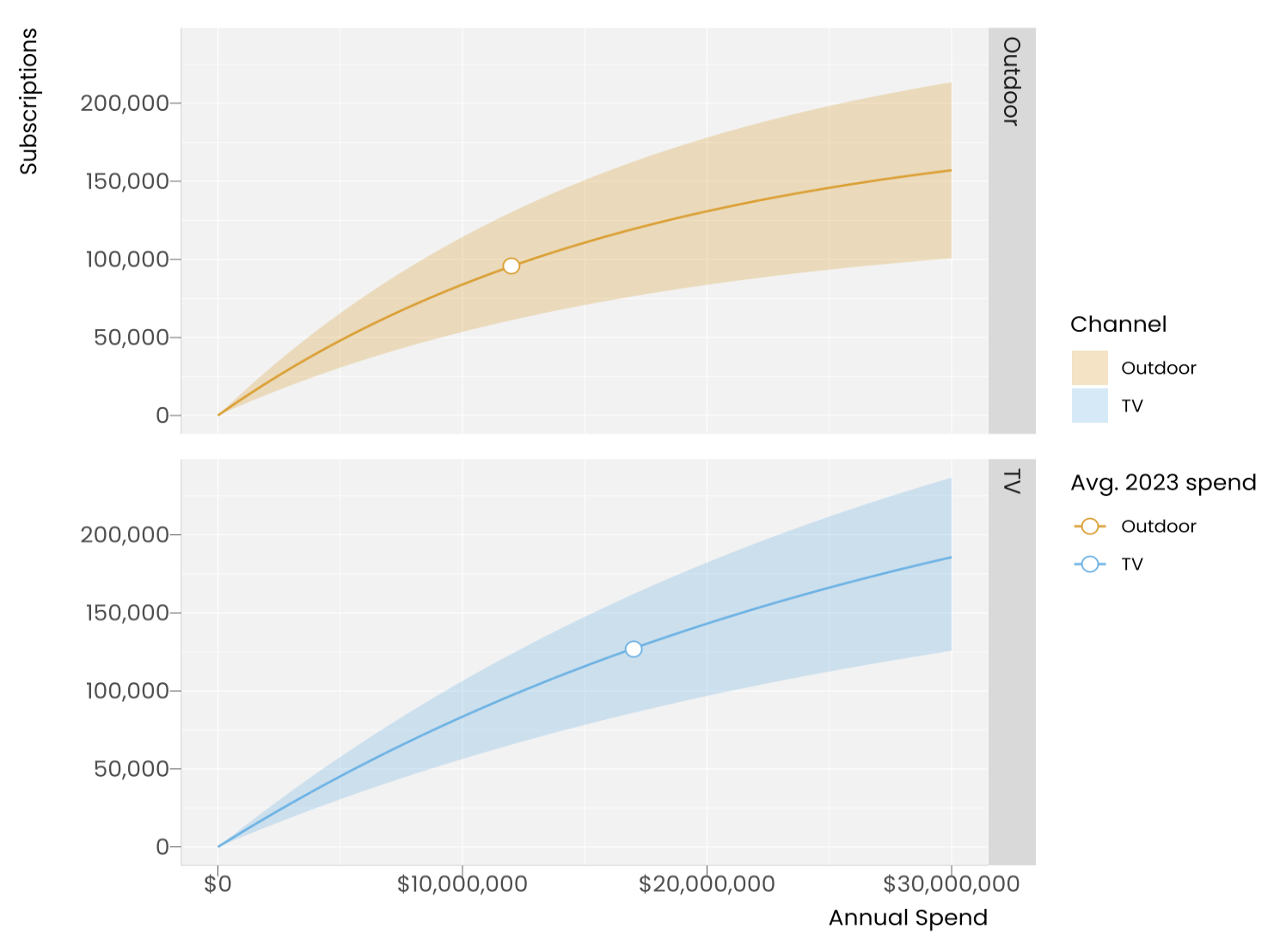
Fig. 1: Prior response curves

Fig. 2: Posterior response curves
Subscriber lifetime value
For subscription businesses, a great approach for estimating customer lifetime value is survival analysis. Making these models Bayesian adds further richness and means we can construct realistic, nuanced models using easy to obtain customer data.
These models generate survival curves. These give the probability that a new subscriber will still be a subscriber at different points in the future.
We can combine this with estimates for revenues and costs to estimate lifetime value.
Because the model is Bayesian, we get a distribution, so we can report things like ‘the probability the CLV is > £175 is 99%’.
See this post for a more in-depth discussion on Bayesian survival models for LTV.

Fig. 3: Survival analysis outputs
Combining posteriors to calculate LTV:CAC
We can combine the outputs from the two models to estimate LTV:CAC. The first model maps the relationship between spend and the (hopefully incremental) number of new subs. The second model tells us how much value we can expect to earn from those subs. Here we assume the only customer acquisition costs are marketing costs - in reality we would probably want to include other costs, e.g. servicing free trials.
How much should we spend on advertising?
In Fig. 4 we’re simulating the impact of spend at different levels on incremental subscriptions and the value they deliver over a 3 year time horizon. We’re then calculating LTV:CAC.
This plot helps us identify budget levels that ensure LTV:CAC is above £1 at different levels of confidence. For example, a risk averse strategy would cap budgets at £10m, giving a 95% chance of a LTV:CAC > £1. Or if we want a likely case strategy, we could set the budget at around £25m.

Fig 4: Spend vs. LTV:CAC
Concluding thoughts
Bayesian models are hugely valuable in business settings because we can construct simulations from the outputs to guide decision making. Here we we’re using two Bayesian models to map out the relationship between total marketing budget and the LTV:CAC ratio, to help inform total annual budgets.